➔ Index of ⦁ Linear Regulators ⦁
Linear regulators - Simplest regulator
Here, the simplest linear regulator is presented to start the analysis of such a type of device
Ideal linear regulator
The simplest linear regulator with ideal components, ideal load and ideal input voltage, is made of a pass device, an error amplifier and a feedback network. But something is missing here! Input and output capacitors? Controller or compensator? Filters? Well, in the ideal world, a linear regulator can be seen just like a variable resistor used to keep the voltage constant at its output node; no external noise can affect its behaviour and all the components in the feedback network don't need tolerance and stray parameters compensations. Moreover, we work under the assumption that the load is constant. In the image below you can find the simplest and most ideal linear regulator possible.
Idealities
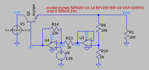
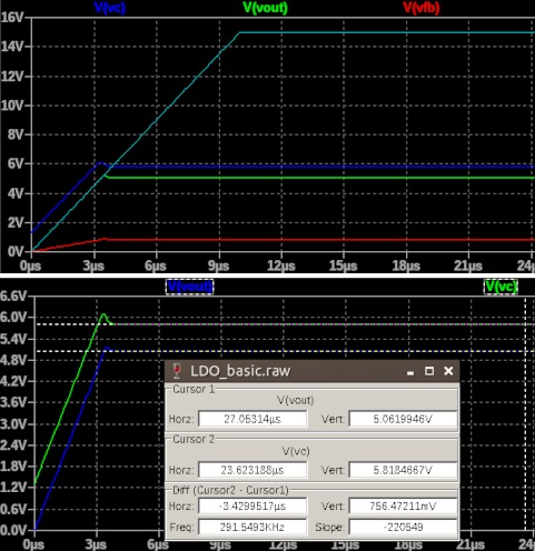
Operational amplifiers are UniversalOpamp1 (Voffset=0V, input resistance=500MOhm, gain-bandwidth product=10M), resistors don't have tolerances, voltage reference is a super accurate and precise, perfectly temperature compensated device, output is a perfect constant resistor, input is constant, no ripple and 0Ohm output impedance, pass device is a very simple NPN bipolar transistor (betaF=200A/A, saturation current=1e-14A, Early voltage=1000V, so, negligible, emitter, collector and base resistance=0Ohm). Now let's see the startup and steady state simulation in the time domain.
Beta-based model
The first model that can be used exploits the transistor beta, assuming that it is fixed and doesn't change under different loading conditions (which means eventually changing the bias point of the bias device). First of all, let's find the input resistance seen by the controller output: $$R_{in} = R_{out}(\beta+1)+R_B$$ Now we have to make an assumption: the vbe threshold voltage has a fixed value that we have to choose $$V_{\gamma} = const,\;typically\;0.7V$$ $$I_B = \frac{V_C}{R_{in}}, \quad I_E=I_{out}=\frac{V_{out}}{R_{out}}=(\beta+1)I_B=(\beta+1)\frac{V_C-V_{\gamma}}{R_{in}}$$ Control voltage instead is defined as (considering also the vbe threshold voltage) $$V_C = -\frac{R_F}{R_S}\frac{R_L}{R_H+R_L}V_{out} + (1+\frac{R_F}{R_S})V_{ref} = -f0*V_{out}+r0*V_{ref}$$ Now we can rearrange the terms; for simplicity we define $$r0 = 1 + \frac{R_F}{R_S}$$ $$f0 = \frac{R_L}{R_H+R_L}\frac{R_F}{R_S}$$ So the final Vout can be written as $$V_{out} = \frac{V_{ref}r0-V_{\gamma}}{\frac{R_{in}}{R_{out}(\beta+1)} + f0}$$
Ebers-Moll based model
The model of such a circuit is pretty simple and a little more accurate than the previous one since vbe is calculated rather than assumed to be a constant value. Let's find the output-to-control function: $$r0 = 1 + \frac{R_F}{R_S}$$ $$f0 = \frac{R_L}{R_H+R_L}\frac{R_F}{R_S}$$ $$V_C = -\frac{R_F}{R_S}\frac{R_L}{R_H+R_L}V_{out} + (1+\frac{R_F}{R_S})V_{ref} = -f0*V_{out}+r0*V_{ref}$$ Now let's calculate the control-to-output function. First of all, let's remember the Ebers-Moll NPN model. $$I_{out} = I_E = I_S(e^{\frac{V_{BE}}{V_T}}-1)(1+\frac{V_{CB}}{V_{AS}}) \quad V_{BE} = V_Tln(\frac{I_E}{I_S(1+\frac{V_{CB}}{V_{AS}})}+1)$$ Then let's find Vout with Kirchoff's voltage law in the Vc, Vbe, Vout loop. $$V_{out} = V_C-V_{BE} = -f0*V_{out}+r0*V_{ref} - V_Tln(\frac{I_E}{I_S(1+\frac{V_{CB}}{V_{AS}})}+1)$$ Now we can remove the Early effect term since it is negligible in these calculations so the final formula is $$V_{out} = \frac{V_{ref}r0 - V_Tln(\frac{I_E}{I_S}+1)}{1+f0}$$ But, hey!, Vout expression depends on Ie=Iout which depends on Vout! The iterative method can be used here to find an accurate value for Vout as you can see in the following paragraph.
Octave simulation script
In the following section you can find the Octave code used to simulate such a circuit; results based on two models are calculated: beta-based (assuming BJT beta and vbe threshold are constants, base resistance is 0) and iterative method-based on Ebers-Moll emitter current model
0
1
2
3
4
5
6
7
8
9
10
11
12
13
14
15
16
17
18
19
20
21
22
23
24
25
26
27
28
29
30
31
32
33
34
35
36
37
38
39
40
41
clear all
close all

% External parameters
Vin = 10
Vout = 5
Rh = 10000
Rl = 2000
Rs = 1000
Rf = 22000
Rb = 0
Vr = 1.06
Rout = 1/(1/100+1/(Rh+Rl)+1/5)
T = 27+273.15

% Pass device properties and constants
Vg = 0.74
beta = 200
k = 1.380649e-23
q = 1.602176634e-19
Vt = k*T/q
Isat = 1e-14

% Calculations using beta
rin = (1+beta)*Rout+Rb;
r0 = 1+Rf/Rs;
f0 = Rl/(Rh+Rl)*Rf/Rs;
printf("---------\n");
Vout = (-Vg+Vr*r0) / (rin/(Rout*(beta+1)) + f0)

% Calculations using an iterative method
Vout2 = 3;
vbe2 = 0.8;
for i=1:10
  Io2 = Vout2/Rout;
  vbe2 = Vt*log(Io2/Isat+1) ;
  Vout2 = (Vr*r0-vbe2) / (1 + f0);
endfor
printf("---------\n");
Io2
vbe2
Vout2
Simulation results
Simulations done with the shown circuit, Vin=15V, varying load, personalized ideal NPN, no Cin, no Cout.
| Octave simulation Ebers-Moll model |
Octave simulation Beta-based model |
LTSpice simulation | |
|---|---|---|---|
| 100Ohm load | 5.0621V | 5.0657V | 5.0620V |
| 5Ohm load | 5.0456V | 5.0657V | 5.0455V |
Ebers-Moll iterative method gives good and accurate results! Moreover, it considers changes of Vout dependent on Iout while the other one always returns the same value (one of the reasons is due to the base resistance set to 0Ohm). However, BJT cannot have 0Ohm base resistance so we have to put some value in our super-ideal NPN model; such non-zero value will change the steady state output voltage under different load conditions (you can explicitly see this dependency in the beta-based model) so we need a different controller. Moreover a non-zero base resistance, in combination with a non-existent output capacitor, can also worsen the step load response, causing a too high voltage drop. These aspects will be discussed in the next article.
Share this page


Comments
Be polite and respectful in the comments section. In case of doubts, read this before posting.
Posted comments ⮧
Comment section still empty.
INDEX
INFO
STATISTICS
PREVIOUS ARTICLE
NEXT ARTICLE
CONTACTS
SHARE