FEMM - Introduction to magnetics

When the program starts, choose "Magnetics problem" from the dropdown list that appears. An empty white screen will appear.

Remember that FEMM is a 2D solver but you need to specify the depth (inside the computer screen) of the structure you are defining to calculate properly some properties. This will be done later.

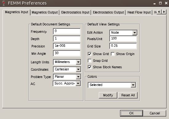
From Edit>Preferences you can change the default values and other properties of your working environment. It is always good to set dimensions to mm and to enable Show Grid, Show Origin and Snap Grid. You can also change the default appearance when creating a new project and finally, you can change the default colors of the various components on the design. You can leave all the other settings unchanged since they will be modified later in the problem definition box.

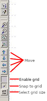
It is very comfortable to have a defined grid in our design and to snap to it so let's define the grid and enable it through the three buttons on the left bar if it is not done by default.

Now let's draw: let's sketch a very simple planar inductor made of two symmetrical 'C' coils, with a perfect linear B-H characteristic and no air gap.

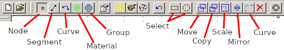
Press the Node button and press the left mouse button on the point of the screen you want to insert the node. If you want to be precise, you can press the TAB key to insert the point coordinates.

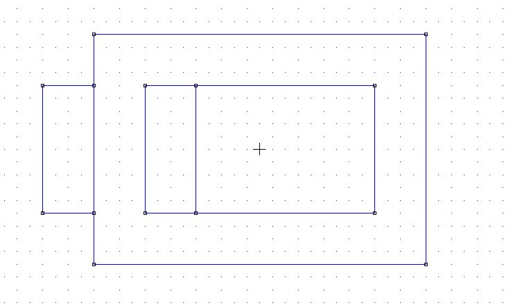
Insert 4 points at the coordinates (-13,9), (13,9) (13,-9) (-13,-9). Then add the other 4 nodes at (-9,5), (9,5), (-9,-5), (9,-5). Now select the Segment button and press the first on the first 4 nodes, two by two to draw an external rectangle; do the same for the inner rectangle. This will be your inductor core section.

Now add two areas to simulate the winding: draw 4 points at (-17,5), (-13,5), (-17,-5), (-13,-5). Add the other two points at (-5,5) and (-5,-5). Connect them to obtain the same figure shown aside.

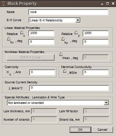
Now we have to define some materials: let's start with the core and make it as simple as possible. Go to Property>Materials and then choose Add Property. Call the new name 'core' and give a relative mu of 1000 for both x and y directions. Keep all the other inputs as by default.

Repeat the same procedure for the coil and for the air: create an 'air' material with all the default values set - don't change anything - and a 'wire' material with 0.5MA/m² as Electrical Conductivity.

Now you can assign the material to various sections of the drawing. Press the Material button in the horizontal bar (the green one ) and put some points in the various areas, then press each of them with the right mouse button and press the spacebar. A Properties

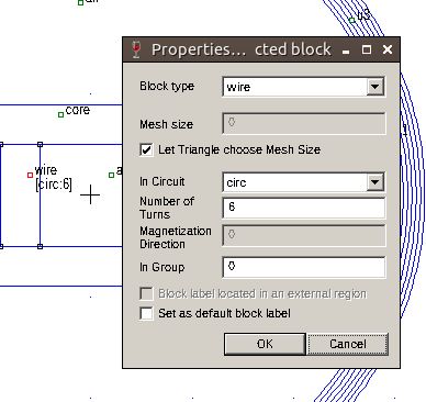
Now go to Properties>Circuits and create a new circuit called 'circ'. Check the 'Series' round button and write 2 in the box (2Amps).

Now you have to assign the material to every part of the drawing: press the Material green button in the top horizontal bar and place a dot in the various sections of the design, as shown. Press LMB on the area, then RMB and then press the spacebar to make the Properties dialogue box appear. In 'Block Type' select the right material; for the wire section (all the wires of the coil are simulated as a homogeneous copper area) you have to add also the circuit in the 'In circuit' box, then specify 6 and -6 for the 'Number of turns'.

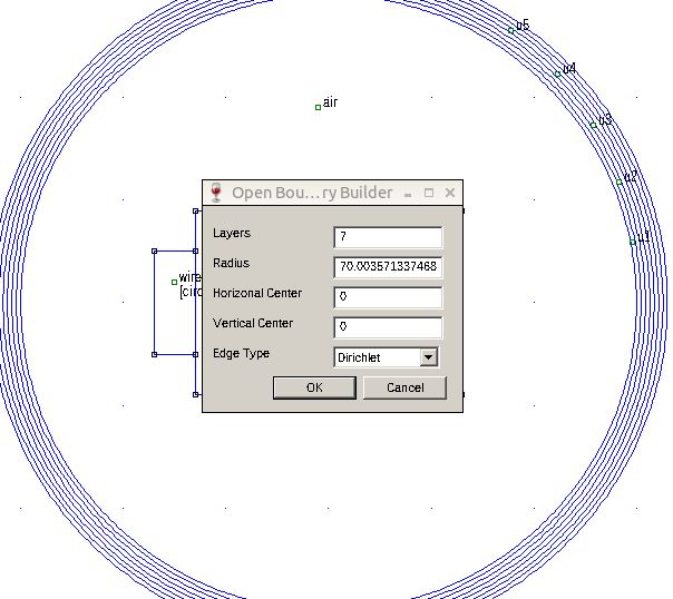
Go to Edit>Creat Open Boundary: the shown label appears. Write the shown values in the boxes then press OK. 7 layers all around the design will be created as a boundary to your design.

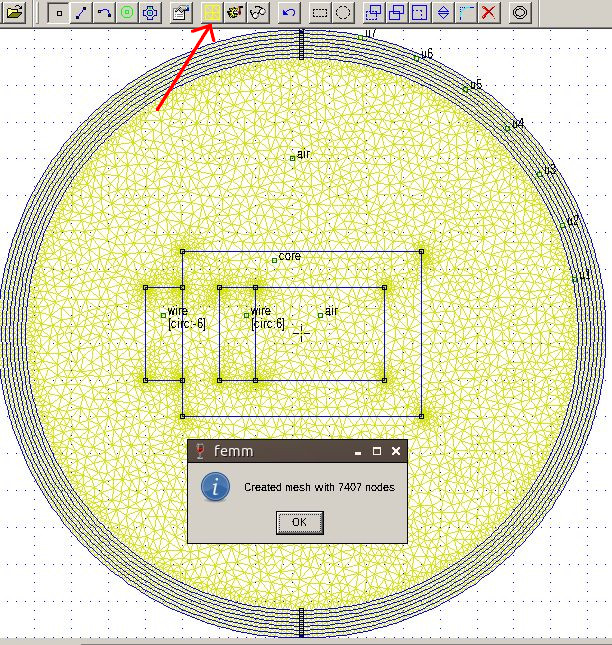
Press the Create Mesh yellow button; if everything went well, a popup should appear, with the number of cells created. If you can't see the mesh, check Mesh>Show Mesh.

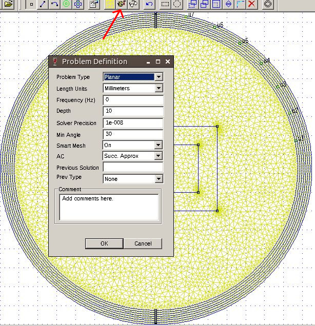
Now you have to set up the simulation environment. Press the 'Problem' button in the menu bar. In the dialog set the values in the box as shown; the meaning of the various labels are briefly explained below.

Now launch the simulation through the pointed button; you should see a fast computation dialogue box appear, and if no error is detected, you can proceed with the post-simulation analysis.

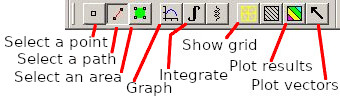
To view the results you have to press the glasses button; a new window will show up. Usually one wants to see how the B and H fields are distributed in the drawn structure and how the current flows in the conductor sections. Let's take a look at the Flux Density. Press the Plot results button and select Flux density (check Show density plot and Show legend): you'll get a result similar to the one shown below; the value of B at the centre of the core is 0.230T more or less and this seems ok also from calculation: $$\Phi \cdot \mathfrak{R} = H \cdot l_m = I \cdot n; \quad H \cdot \mu \cdot A_c = B \cdot A_c=\Phi$$ Rearranging terms one obtains $$B=\frac{I \mu n}{l_m}$$ $$B=\frac{6turns \cdot 2A \cdot 4\pi10^{-7} \cdot 1000}{2 \cdot 0.01mm + 2 \cdot 0.018mm + 2\pi \cdot 0.002mm} = 0.220T$$ The calculated value is very similar to the B field at the centre of the core, obtained from simulation. In the calculation, l_m (mean magnetic path length) is calculated approximating edges as a quarter of a circle.

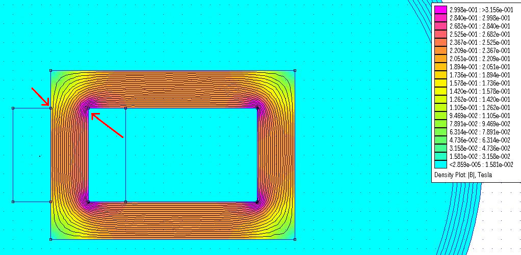
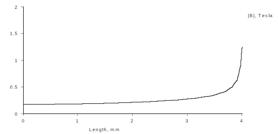
B distribution is not uniform across the section, it is sensibly higher at inner corners; to properly evaluate B values it is good to have a linear plot of B along the section of the core. To do this, press the Select path button and highlight the two points marked in the image, then press the Graph button and select |B| Magnitude of flux density. A new window will appear and the plot will be shown.

This is just the first introduction to FEMM with a very basic example. We performed a DC analysis of a core whose conductivity has been set to 0MS/m, no lamination defined, perfectly linear and isotropic magnetic material: this wouldn't be a complete tutorial on magnetics but just a recap on the main FEMM functions and features; now you should have an idea of the power of this apparently simple and intuitive free tool :)