Transmission lines - Part IV: Time domain

Transmission line analysis in the time domain is very difficult so frequency domain analysis is always preferred. However, sometimes the engineer wants to see what is happening on the line over time and how the signal is reflected at the source, looking at the signal shape, ringing, rise and fall times, overshoot and so on: this is quite impossible to do by hand but we can still understand how reflections happen in the channel by referring to the 'bounce diagram'.

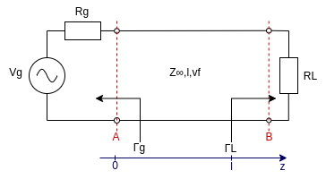
The transmission line model is given and the various impedances are known; we have to determine the shape of the voltage waveform at the receiver and eventually at the transmitter given an input signal (usually a step). At the instant 0s such step is applied to the input of the transmission line and the voltage is: $$v_{tx}(t) = \frac{Z_0}{Z_0+Z_{g}} u(t) = e(t)$$ After a well-defined time interval, the signal reaches the other end of the channel and, just an infinitesimal instant before being reflected or absorbed, the voltage at the receiver is: $$v_{1rx,b}(t) = e(t-\tau)$$ and the time interval is defined as: $$\tau=\frac{L}{v_f}$$ Now the signal strikes against the receiver interface: its behaviour is determined only by the load impedance and so by the value of the reflection coefficient. In general, the value of the signal, an infinitesimal instant after the reflection, is: $$v_{1rx,a}(t) = e(t-\tau) + \Gamma_{rx} e(t-\tau)$$ The signal is now sent back to the receiver: $$v_{1tx,b}(t) = e(t) + \Gamma_{rx} e(t-2\tau)$$ Here the signal finds the output impedance of the transmitter and so we get another reflection here: $$v_{1tx,a}(t) = e(t) + \Gamma_{rx} e(t-2\tau) + \Gamma_{tx}\Gamma_{rx} e(t-2\tau)$$ Again, the signal goes towards the receiver and the signal here becomes: $$v_{2rx,b}(t) = e(t-\tau) + \Gamma_{rx} e(t-\tau) + \Gamma_{tx}\Gamma_{rx} e(t-3\tau)$$ This procedure can be repeated forever.

For a simple case like this one we can easily see that the voltage at the transmitter and the receiver can be written as follows: $$v_{tx}(t) = e(t) + \Gamma_{rx}e(t-2\tau) + \Gamma_{rx}\Gamma_{tx}e(t-2\tau) + \Gamma_{rx}^2\Gamma_{tx}e(t-4\tau) + \Gamma_{rx}^2\Gamma_{tx}^2e(t-4\tau)...$$ $$v_{tx}(t) = \frac{Z_0}{Z_0+Z_{g}}\left[\sum_{n=0}^\infty \Gamma_{rx}^n \Gamma_{tx}^n u(t-2n\tau) + \sum_{n=0}^\infty \Gamma_{rx}^{n+1} \Gamma_{tx}^n u(t-2n\tau)\right]$$ $$v_{tx}(t) = \frac{Z_0}{Z_0+Z_{g}}\left[\sum_{n=0}^\infty \Gamma_{rx}^n \Gamma_{tx}^n u(t-2n\tau) + \Gamma_{rx} \sum_{n=0}^\infty \Gamma_{rx}^{n} \Gamma_{tx}^n u(t-2n\tau)\right]$$ $$v_{rx}(t) = e(t-\tau) + \Gamma_{rx}e(t-\tau) + \Gamma_{rx}\Gamma_{tx}e(t-3\tau) + \Gamma_{rx}^2\Gamma_{tx}e(t-3\tau) + \Gamma_{rx}^2\Gamma_{tx}^2e(t-5\tau)...$$ $$v_{rx}(t) = \frac{Z_0}{Z_0+Z_{g}}\left[\sum_{n=0}^\infty \Gamma_{rx}^n \Gamma_{tx}^n u(t-(2n+1)\tau) + \sum_{n=0}^\infty \Gamma_{rx}^{n+1} \Gamma_{tx}^n u(t-(2n+1)\tau)\right]$$ $$v_{rx}(t) = \frac{Z_0}{Z_0+Z_{g}}\left[\sum_{n=0}^\infty \Gamma_{rx}^n \Gamma_{tx}^n u(t-(2n+1)\tau) + \Gamma_{rx} \sum_{n=0}^\infty \Gamma_{rx}^{n} \Gamma_{tx}^n u(t-(2n+1)\tau)\right]$$ Now it is possible to find the steady state behaviour of the voltage at the rx and tx points of the transmission line. Remember that $$\sum_{n=0}^\infty x^n = \frac{1}{1-x}$$ so we can rewrite the previous equations like $$v_{tx} = v_{rx} = U \frac{Z_0}{Z_0+Z_{g}} \left[\sum_{n=0}^\infty (\Gamma_{rx} \Gamma_{tx} )^n + \Gamma_{rx} \sum_{n=0}^\infty (\Gamma_{rx} \Gamma_{tx} )^n \right]$$ $$v_{tx} = v_{rx} = U \frac{Z_0}{Z_0+Z_{g}} \frac{1+\Gamma_{rx}}{1-\Gamma_{rx} \Gamma_{tx}}$$

Let's solve an example with the following values: $$R_g = 50Ohm \quad Z_0 = 50Ohm \quad R_l = 50Ohm \quad V_g = 5V $$ Now we have to find the reflection coefficient at the generator and the load $$\Gamma_{rx} = \frac{R_l - Z_0}{R_l + Z_0} = 0$$ $$\Gamma_{tx} = \frac{R_g - Z_0}{R_g + Z_0} = 0$$ Now we calculate the v_tx which is the magnitude of the voltage at the input of the line as soon as the generator is enabled. $$v_{tx} = \frac{Z_0}{Z_0+R_g} V_g = 2.5V$$ Since the reflection coefficient at the load is 0, there will be no reflected wave. In this matched impedance condition, there is no superimposition between forward and backward travelling waves so no distortion is visible at both ends. This is an ideal and preferred condition for all the transmission lines.

Solve using the following values: $$R_g = 50Ohm \quad Z_0 = 100Ohm \quad R_l = 25Ohm \quad V_g = 5V \quad v_f = 2 \cdot 10^8 \frac{m}{s} \quad L = 20m$$ Let's calculate the time of flight between the source and the load $$\tau = \frac{L}{v_f} = 100ns$$ Now we calculate the reflection coefficients $$\Gamma_{rx} = \frac{R_l - Z_0}{R_l + Z_0} = -0.6$$ $$\Gamma_{tx} = \frac{R_g - Z_0}{R_g + Z_0} = -0.33$$ Now we calculate the v_tx which is the magnitude of the voltage at the input of the line as soon as the generator is enabled. $$v_{tx} = \frac{Z_0}{Z_0+R_g} V_g = 3.33V$$ Now we calculate v_1,rx $$v_{1,rx,b} = v_{tx}(t-\tau) = 3.33V(t-100ns)$$ When the signal arrives at the load, it is reflected back generating another pulse with the following characteristic $$v_{1,rx,a} = v_{1,rx,b} \cdot \Gamma_{rx} = -2V(t-100ns)$$ Let's calculate the next steps $$v_{1,tx,b} = v_{1,rx,a}(t-100ns) = -2V(t-200ns)$$ $$v_{1,tx,a} = v_{1,tx,b} \cdot \Gamma_{tx} = 0.67V(t-200ns)$$ $$v_{2,rx,b} = v_{1,tx,a}(t-100ns) = 0.67V(t-300ns)$$ $$v_{2,rx,a} = v_{2,rx,b} \cdot \Gamma_{rx} = -0.40V(t-300ns)$$ $$v_{2,tx,b} = v_{2,rx,a}(t-100ns) = -0.40V(t-400ns)$$ $$v_{2,tx,a} = v_{2,tx,b} \cdot \Gamma_{tx} = 0.132V(t-400ns)$$ $$v_{3,rx,b} = v_{2,tx,a}(t-100ns) = 0.132V(t-500ns)$$ $$v_{3,rx,a} = v_{3,rx,b} \cdot \Gamma_{rx} = -0.079V(t-500ns)$$ $$v_{3,tx,b} = v_{3,rx,a}(t-100ns) = -0.079V(t-600ns)$$ $$v_{3,tx,a} = v_{3,tx,b} \cdot \Gamma_{tx} = 0.026V(t-600ns)$$ $$v_{4,rx,b} = v_{3,tx,a}(t-100ns) = 0.026V(t-700ns)$$ $$v_{4,rx,a} = v_{4,rx,b} \cdot \Gamma_{rx} = -0.016V(t-700ns)$$

The voltage at tx is 3.33V, 2V, 1.732V, 1.679V.
The voltage at rx is 1.33V, 1.6V, 1.653V, 1.663V.
The steady-state value of the voltage over the transmission line is 1.666V and this can be easily calculated as the voltage when the frequency is 0Hz: the transmission line behaves like a short circuit and the voltage is $$V_i = V_o = V_{line}(z) = V_g \frac{R_l}{R_l+R_g}$$

Now you can simulate the circuit and check if the results are correct. For this purpose, I use QUCS, a versatile, free and open-source SPICE-based simulator, oriented to RF simulations. Down below you can find both the circuit and the results. You can see that the steps have the same values as calculated.

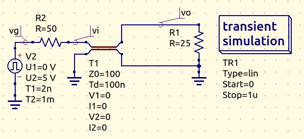
Remember to set the transmission line Td property (delay time) to 100ns.

Note how the voltage at tx(vi) changes every 200ns starting from 0ns while at rx(vo) it changes every 200ns but with a delay of 100ns.