Transmission lines - Part VI: Smith chart

To analyse the behaviour of voltage and current along a transmission line, it is good practice to calculate impedances or reflection coefficient at main sections (line start, line end, impedance mismatch section, stub). To do this, few different approaches may be used, according to the required precision and the available instrumentation.

The Smith Chart allows to find the impedance at any section of a transmission line using a geometrical approach, with only few calculations.

Before introducing the Smith Chart, we have to understand how to normalize the quantities we deal with, mainly the impedance and the length of the various segments of the transmission line. Here one can see the definition of normalized impedance (in relation to the line characteristic impedance) and normalized length (in relation to the signal wavelength), respectively. $$\mathfrak{z}(z) = \frac{Z(z)}{Z_{\infty}}$$ $$\mathfrak{z}(z)=\frac{\mathfrak{z}(0)-jtan(kz)}{1-j\mathfrak{z}(0)tan(kz)}$$ Another quantity to be normalized when using the Smith Chart is the length, calculated as $$\mathfrak{l} = \frac{l}{\lambda}$$ Then, the reflection coefficient can be written as: $$\Gamma(z)=\frac{\mathfrak{z}(z)-1}{\mathfrak{z}(z)+1}$$

If you want, you can write a script to calculate the impedance at any z section of the line using the given formula. However, if you don't have a calculator, the Smith Chart will help you in the task.

Here is the Smith Chart: let's see how it is made and how to use it.

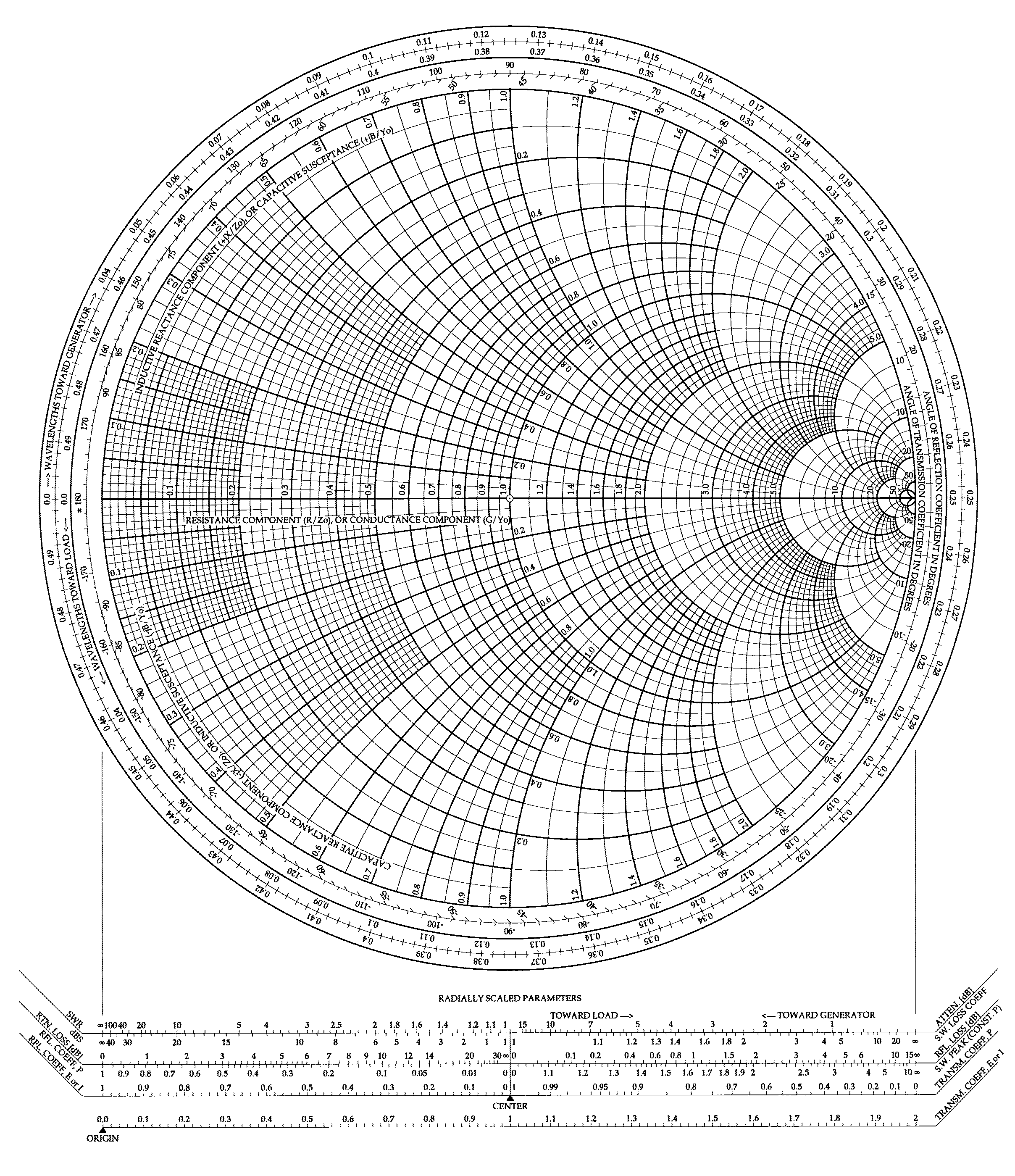
On the horizontal line in the middle, one can find values for the normalized resistance, whereas along the circles are the imaginary terms. The upper half circle is used for positive imaginary terms (inductive component) and the lower one for negative terms (capacitive component).

Knowing the normalized length (dimensionless number obtained as ratio between physical length of the transmission line and wavelength of the travelling wave), one can easily find the impedance in a generic section z, knowing the impedance in another point of the line. Let's proceed with an example where the impedance at .

A transmission line has the following properties $$l = 30cm = 0.3 m \quad (physical \ length)$$ $$f = 14 GHz \quad (signal \ frequency)$$ $$Z_0 = 50 Ohm \quad (characteristic \ impedance)$$ $$Z_L = 25-j10 Ohm \quad (load \ impedance)$$ $$\varepsilon_r = 3$$ I need to calculate the wavelength of the signal in the medium $$\lambda = \frac{c}{f\sqrt(\varepsilon_r)} = 0.012363 m$$ Let's calculate the normalized impedance and the normalized length $$\mathfrak{z}_L = \frac{25-j10}{50} = 0.5-j0.2$$ $$\mathfrak{l} = \frac{l}{\lambda} = 24.265$$ We are interestend only in the residual length, so let's consider only the 0.265 as normalized length. Now, let's draw a dot (dark red) on the Smith Chart at the calculated normalized impedance and draw a circle (green) whose radius is given by the distance between 1+j0 and the point 0.5-j0.2. Trace a line passing across this point and 1+j0 (dark blue). The line intersects the outer circle with numbers from 0.0 to 0.49: the value is around 0.459.

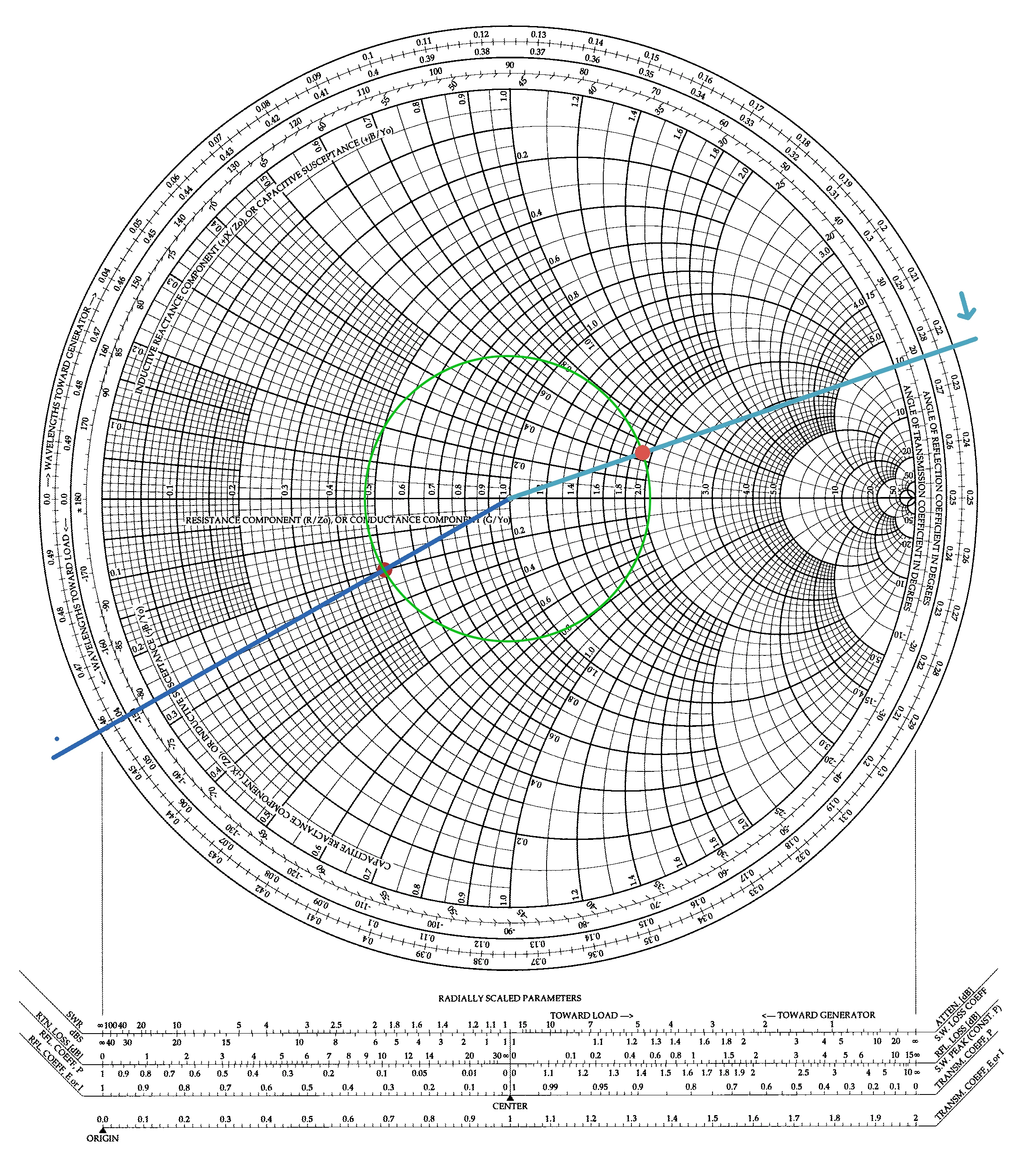
Now we have to move from the load to the generator (clockwise direction, as suggested from the chart itself) of 0.459+0.265; this gives 0.724, which is higher than 0.5 so we have to subtract it, obtaining 0.224. This is the normalized length at the generator section. Let's draw a line (light blue) from this point on the outer circle and 1+j0: the intersection of this line with the (green) circle is the value of the normalized impedance at the generator (light red dot). The value is 1.92+j0.47.

The impedance at the generator section is $$Z_G = Z_0 \cdot \mathfrak{z}_G = 50 \cdot (1.92+j0.47) = 96 + j23.5 Ohm$$

We can check the result using the formula, which gives 97.17 + j24.35 Ohm. As you can see, Smith Chart method is good to quickly check the your calculations but not so precise.