Control theory - From formulas to Bode plot

A transfer function is analysed in the frequency domain to get information about its response for sinusoidal inputs. This concept is very important: the whole analysis of a dynamic system is based on this assumption.

A sinusoidal input allows to completely characterise the system in the frequency domain in the same way as a unitary step input allows to completely characterise the system in the time domain. This holds true since a sinusoidal input (at a fixed frequency) is equivalent to a Dirac's delta function in the frequency domain, so, system response analysis is equivalent to evaluating the transfer function in frequency domain at that frequency.

But which is the physical meaning of a transfer function? How can we relate zeros (values of frequency that null the output) and poles (values of frequency that make the output unbound) with the real behaviour of a system in the time domain?

When studying a transfer function in the frequency domain, we can see that numerator and denominator are polynomials with 's' as complex variable. Since 's' is a generic complex number, we can say that $$s = \sigma + j\omega$$ where σ is the real part and ω is the imaginary part. All zeros and poles can be plotted on a zero-pole plane where the y axis is jω and the x axis is σ, identifying poles with an 'X' and zeros with an 'O'. Let's consider again the previous example (the RC filter) and recall the state equation: $$\frac{dv_O(t)}{dt} = -\frac{1}{RC}v_O(t) + \frac{1}{RC}v_I(t)$$ This is an Oridnary Differential Equation whose form is $$y'(t) = f(t)y(t) + g(t)$$ and the general solution is $$y(t) = ce^{\int f(t) dt} + e^{\int f(t) dt} \int g(t)e^{-\int f(t) dt} dt$$ Now, since the target consists in the evaluation in the frequency domain of the transfer function, all we have to do is applying a purely and unitary sinusoidal input to the system and finding the output. $$v_I(t) = e^{j\omega t} = cos(\omega t) + j sin(\omega t)$$ The state equation becomes $$\frac{dv_O(t)}{dt} = -\frac{1}{RC}v_O(t) + \frac{1}{RC}e^{j\omega t}$$ Knowing that $$y(t) = v_O(t)$$ $$\int f(t) dt = -\frac{1}{RC}t$$ $$g(t) = \frac{1}{RC}e^{j\omega t}$$ the solution is then (follow the passages) $$v_O(t) = ce^{-\frac{1}{RC}t} + e^{-\frac{1}{RC}t} \frac{1}{RC} \int e^{j\omega t}e^{\frac{1}{RC}t} dt$$ Note! 'c' is 0 but the term inside the integral is ... the Laplace transform with σ set to 0! Here you see, finally, the relationship between the differential equations governing a system and their form in the Laplace domain. $$v_O(t) = e^{-\frac{1}{RC}t} \frac{1}{RC} \int e^{t(j\omega + \frac{1}{RC})} dt$$ $$v_O(t) = e^{-\frac{1}{RC}t} \frac{1}{RC} \frac{1}{j\omega + \frac{1}{RC}}e^{t(j\omega + \frac{1}{RC})}$$ $$v_O(t) = \frac{1}{RC} \frac{1}{j\omega + \frac{1}{RC}}e^{j\omega t}$$ $$v_O(t) = \frac{1}{RC} \frac{\frac{1}{RC} - j\omega }{\frac{1}{(RC)^2} + \omega^2}e^{j\omega t}$$ Remember how v_I(t) was defined, let's find h(t) and compare this result in the time domain with the one in frequency domain obtained using Laplace transform $$h(t) = \frac{v_O(t)}{v_I(t)} = \frac{1}{RC} \frac{\frac{1}{RC} - j\omega }{\frac{1}{(RC)^2} + \omega^2} \qquad H(s) = \frac{V_O(s)}{V_I(s)} = \frac{1}{RC} \frac{1}{s+\frac{1}{RC}}$$ Can you see it? They are the same!

After all that math you should note that the imaginary term jω appearing in the transfer function in time domain is there since we posed e^jωt as input, a pure sine input! This is important to understand where the gain-phase plots come from and why we neglect some parts of the zero-pole diagram. Moreover, from this results we see that the transfer function in frequency domain is obtained posing $$s = j\omega$$ σ is neglected! This is done since we are not interested in exponentially decaing or growing inputs, but only in a simple sine input!

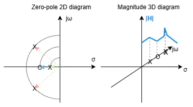
Look at the image aside: now you should understand where the gain plot (that is the first part of the Bode plot) comes from! It's a projection of the 2D zero-pole diagram on the jω axis and the evaluation of such projection for every value of ω from 0 to infinity. We neglect other planes for σ different than 0 since they correspond to input that are not pure sine.

Moreover, we said that zeros are the place where H becomes 0 and poles where H becomes infinity, however from the gain plot we don't see these values much often. This happens because we are seeing the effect on |H| only along the jω axis. A plot of the gain will be exact 0 only in the origin (jω=0 because there is a zero in (0,0)) and infinity only with purely complex conjugated poles (poles lying on the jω axis, with no real part). Look at the picture: the two poles are not purely complex so the gain won't go to infinity , the single pole is real so, again, |H| won't be infinity and the zero is not in (0,0) so |H| won't be 0 in that point.

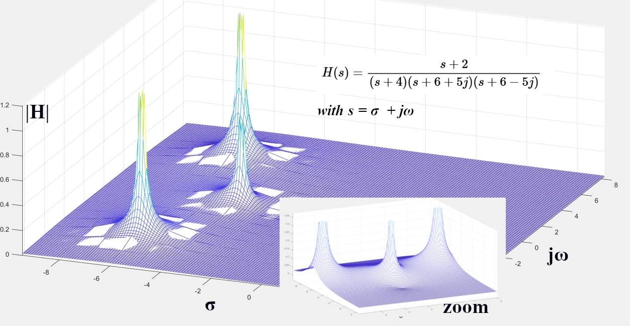
Look at the image below: a zero-pole-gain plot is shown with a zoom to make the zero more visible. The plotted function is $$H(\sigma + j\omega) = \frac{\sigma + j\omega + 2}{(\sigma + j\omega + 4)*( \sigma + j\omega + 6 + 5j)*(\sigma + j\omega + 6 -5j)}$$ You can see how the complete 3D function goes to 0 and infinity.

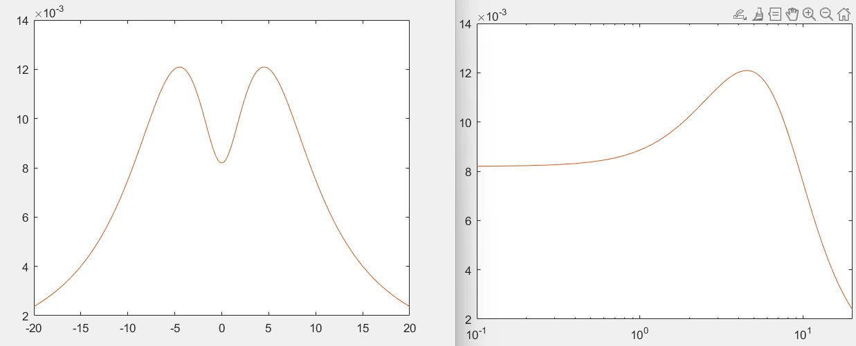
We have seen that the 3D plot contains a lot of information along the σ axis too, but we want to neglect it because this contribution is not relevant for our system analysis. How to simplify all the previous formulas? Quite simple! Let's remove the σ and we get $$H(j\omega) = \frac{j\omega + 2}{(j\omega + 4)*(j\omega + 6 + 5j)*(j\omega + 6 -5j)}$$ Now that the formula has just one variable, it can be plotted along the jw axis. Since there is no meaning for a negative frequency, only the positive half is considered.

A generic transfer function can be written in a Zero-Pole-Gain form (often referred to as ZPK form). $$H(s) = K \frac{(s+z_1)(s+z_2)+...+(s+z_n)}{(s+p_1)(s+p_2)+...+(s+p_n)}$$ When writing down a transfer function, it is warmly recommended to use this form since it highlights the value of zeros, poles and DC gain, simplifying the analysis.